
Structural Analysis - Variographic Models

Structural analysis is crucial for understanding the behavior of regionalized variables. After calculating the experimental variogram, as we saw in a previous post, the next step is to model this behavior using a modeled variogram. In this article, we explore the basics of these models.
Once the experimental variogram is obtained, a modeled variogram is constructed by selecting from a series of admissible models. Key features of a variogram model include:
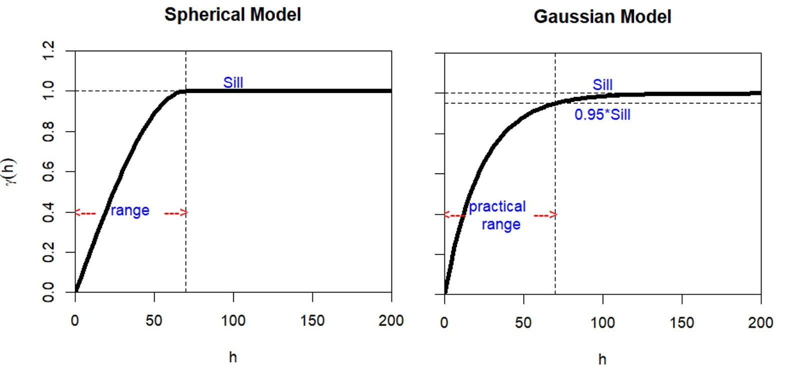
The variogram is zero at the origin.
The variogram gradually increases until reaching a maximum value or sill, except in cases where it increases indefinitely.
The distance at which the variogram reaches the sill is known as the range.
When the variogram is asymptotic concerning the sill, a practical range is defined, representing the distance at which the variogram equals 95% of the sill.
The figure illustrates a spherical and Gaussian variogram model, identifying the main components of each variogram model.
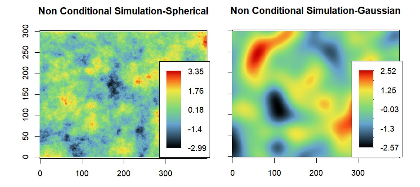
The left figure presents a simulation of the type of regionalized variable associated with the spherical variogram from the example. On the other hand, the right figure shows the corresponding view of the Gaussian variogram.
In conclusion, properly modeling experimental variograms is fundamental for accurately interpreting spatially structured data.
If you are interested in more information on this topic or how to apply these concepts to your project, feel free to contact us at contacto@m2p.cl
References:
Armstrong, M., Basic Linear Geostatistics, 1998, Springer Berlin Heidelberg.
Emery, X., 2013. Geoestadística. Universidad de Chile, Santiago, Chile.
MINES ParisTech / ARMINES (2020). RGeostats: The Geostatistical R Package. Version: 12.0.1. Free download from: http://cg.ensmp.fr/rgeostats.